3.2. Overall workflow

1. Compute HRU (Hydrologic Response Unit, or simply catchment) mean runoff [m/s]

2. Perform overland routing with HRU mean runoff as an input to compute lateral runoff (\(R_{lat}\)) [m/s]

3. Convert \(R_{lat}\) from depth unit to volume (lateral runoff times HRU area) to get lateral discharge (\(q_{lat}\)) [m3/s]

4. Route lateral discharge at each river reach through river network.

The overland routing is optional, and currently simple unit hydrograph based on gamma distribution is used to delay instantaneous runoff.

3.3. River routing schemes

For river reach routing, mizuRoute include five different routing methods. The routing method(s) are applied to each river reach to compute outflow from the reach. The methods are Impulse response function (routOpt=1 in mizuRoute), Lagrangian kinmatic wave (routOpt=2), Euler kinematic wave (routOpt=3), Muskingum Cunge (routOpt=4)), and Diffusive wave (routOpt=5).

This section describes each scheme including numerical implementation. Impulse response function and lagrangian kinematic wave, implemented eariler, are also described in Mizukami et al. (2016). The othter schemes were implemented afterwards, and described in appendices of Cortes-Salazar et al. (2023) (except for Euler kinematic wave).

A fundamental equations for river reach routing start with Saint-Venant equations that consists of two equations

(3.3.1)\[\frac{\partial Q }{\partial x} + \frac{\partial A }{\partial t} = q_{lat}\]

(3.3.2)\[\frac{\partial Q }{\partial t} + \frac{\partial }{\partial x}(\frac{Q^{2}}{A}) + gA\frac{\partial h }{\partial x} = gA(S_{0}-S_{f})\]

where Q is a discharge [m³/s] at time t and a point of reach x, A is a flow cross-sectional area [m²], h is flow height [m], \(S_{0}\) is a slope of reach [m/m], \(S_{f}\) is a friction slope [m/m]. LHS of (3.3.2) consists of advection, inertia, and pressure gradient from the 1st to 3rd terms, while force temrs of RHS of (3.3.2) consists of gravity and frictional force from a river bed.

The frictional slope is written as:

(3.3.3)\[S_{f} = \frac{Q^2}{K^2}\]

(3.3.4)\[K = \frac{A}{n}R^{\frac{2}{3}}\]

where K (Eq. (3.3.4)) is a channel conveyance. n is manning coefficient [-] and R is hydraulic radius [m].

If advection and inertia terms are neglected (i.e., the 1st and 2nd terms in LHS of (3.3.2)) and without lateral flow in (3.3.1), 1-D Saint-Venant equation (3.3.1) and (3.3.2) is reduced to

(3.3.5)\[\frac{\partial Q }{\partial t} + C\frac{\partial Q}{\partial x} = D\frac{\partial^2 Q}{\partial^2 x}\]

(3.3.6)\[C = \frac{1}{K}\frac{\partial K}{\partial A}\]

(3.3.7)\[D = \frac{K^2}{2QB}\]

where C (Eq. (3.3.6)) is a wave celerity [m/s] and D (Eq. (3.3.7)) is a diffusivity [m²/s]. B is a top width of flow cross-sectional area [m].

If D is set to zero (i.e., diffusion is neglected), Eq. (3.3.5) becomes kinematic wave equation. The other way to derive kinematic wave equation is to neglect pressure gradient term in addition to advection and inertia and pressure gradient terms (i.e., all the terms in LHS of Eq. (3.3.2)).

Eq. (3.3.5) serve a starting point of numerical implementation of Impulse response function (section Section 3.3.1), Euler Kinematic wave (section Section 3.3.3), Muskingum-Cunge (section Section 3.3.4), Diffusive wave schemes (section Section 3.3.5).

The numerical implementations of Euler kinematic wave and Diffusive wave are essentially identical. Therefore, a user is referred to section Section 3.3.5 for Euler kinematic wave numerical schemes.

3.3.1. Impulse response function

3.3.2. Lagrangian kinmatic wave

3.3.3. Euler kinmatic wave

See section Section 3.3.5 for details on numerical implementatin of Euler kinematic wave.

3.3.4. Muskingum-Cunge

Muskingum-Cunge (M-C) routing formulation begins with a kinematic wave equation, (3.3.5) with D set to zero. The kinematic wave equation can be discretized with weight factors X and Y to give:

(3.3.4.1)\[\frac{X(I_{t+1}-I_{t})+(1-X)(O_{t+1}-O_{t})}{\Delta t} + C \frac{Y(O_{t}-I_{t})+(1-Y)(O_{t+1}-I_{t})}{\Delta x}=0\]

where \(I_{t+1}\) and \(I_{t}\) are inflow to a reach segment (length is \(\Delta x\)) at the end and beginning of the time step (time step is \(\Delta t\) ) and \(O_{t+1}\) and \(O_{t}\) are outflow from a reach segment at the end and beginning of the time step. The spatial weight factor Y is set to 0.5 and then Eq. (3.3.4.1) is rearranged, giving:

(3.3.4.2)\[O_{t+1} = \frac{-X+0.5 C_{n}}{1-X+0.5 C_{n}} I_{t+1} + \frac{X+0.5 C_{n}}{1-X+0.5 C_{n}} I_{t} + \frac{1-X-0.5 C_{n}}{1-X+0.5 C_{n}} O_{t}\]

where \(C_{n}\) is Courant Number defined by \(C \frac{\Delta t}{\Delta x}\). Eq (3.3.4.2) is generally called Muskingum equation, but Cunge (1969) found that the numerical diffusion in the explicit solution of Eq (3.3.4.2), which can happen depending on weight factors, can match the physical diffusion by setting X (along with Y=0.5) to:

(3.3.4.3)\[X=0.5(1-\frac{Q}{BS_{0} C\Delta x})\]

where \(S_{0}\) is the reach slope, B is a top widith of flow cross-section area. Here discharge Q and B can be estimated by 3-point Q values (\(I_{t+1}\), \(I_{t}\), and \(O_{t}\)). Note that B is a function of Q given channel cross-section assumption (see section x-x). At every time step and reach, temporal weight factor X is update based on given 3-point discharge values. Since Muskingum-Cunge is explicitly solved, the solution can be unstable. To stabilize the solution, the sub time step (\(\Delta t\)) is determined at every simulation step so that the Courant number is less than unity

3.3.5. Diffusive wave

To solve the diffusive wave equation for discharge Q, Eq. (3.3.5) is discretized using weighted averaged finite-difference approximations across two time steps in space (Figure 1; i.e., second-order central difference in the RHS of (3.3.5) and first-order central difference for the second term of the LHS of (3.3.5)).

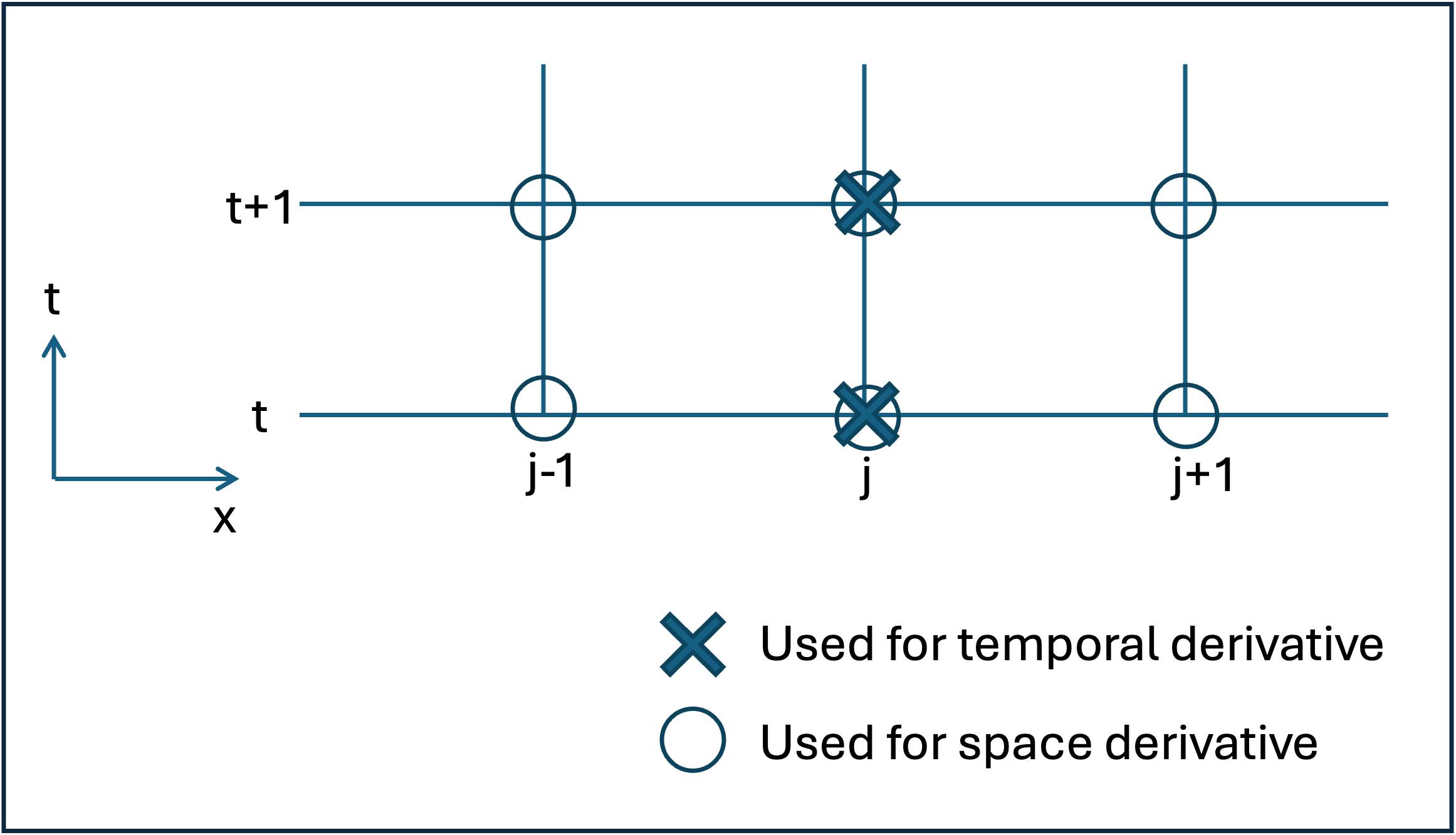
Figure 3.3.5.1 Space and time discretization used for numerical solution of diffusive wave equation

The resulting discretized diffusive wave equation becomes:

(3.3.5.1)\[\begin{split}\frac{Q_{j}^{t+1} - Q_{j}^{t}}{\Delta t} + \frac{C}{2 \Delta x} \cdot ((1- \alpha )(Q_{j+1}^{t} - Q_{j-1}^{t})+ \alpha (Q_{j+1}^{t+1} - Q_{j-1}^{t+1})) = \\\\ D \cdot (\frac{(1- \beta)(Q_{j+1}^{t} - 2Q_{j}^{t} + Q_{j-1}^{t})}{(\Delta x)^2} + \frac{\beta (Q_{j+1}^{t+1} - 2Q_{j}^{t+1} +Q_{j-1}^{t+1})}{(\Delta x)^2})\end{split}\]

Rearranging Eq. (3.3.5.1) to:

(3.3.5.2)\[ \begin{align}\begin{aligned}\begin{split}( \alpha C_{a} - 2 \beta C_{d}) \cdot Q_{j+1}^{t+1} + (2+4 \beta C_{d}) \cdot Q_{j}^{t+1} - ( \alpha C_{a} + 2 \beta C_{d}) \cdot Q_{j-1}^{t+1} = \\\\ -[(1- \alpha )C_{d} - 2(1- \beta )C_{d})] \cdot Q_{j+1}^{t} \\\\ + [2-4(1- \beta )C_{d}] \cdot Q_{j}^{t} \\\\ + [(1- \alpha )C_{a} + 2(1- \beta )C_{d})] \cdot Q_{j-1}^{t} \\\\\end{split}\\C_{a} = \frac{C \Delta t}{ \Delta x}, C_{d} = \frac{D \Delta t}{( \Delta x)^{2}}\end{aligned}\end{align} \]

where \(\alpha\) is the weight factor for the first-order space difference approximation of the second term of the LHS of (3.3.5), and \(\beta\) is a weight factor for the second-order space difference approximation in RHS of (3.3.5). If both weights are set to 1, the finite difference becomes a fully implicit scheme, while setting both weights to zero results in a fully explicit scheme. For default, mizuRoute uses a fully implicit finite-difference approximation (i.e., \(\alpha\) = \(\beta\) = 1). Note that celerity (C) and diffusivity (D) include Q, which means the diffusive equation is actually non-linear. Here celerity (C) and diffusivity (D) are updated at every time step based on the discharges (Q) and flow area (A) at previous time step to liearize the diffusive equation. Note that IRF routing is also based on diffusve equation. a major difference is that in IRF routing, celerity and diffusivity are provided as model parameters and constant in time, though they can be spatially distributed.

To apply the numerical solution of discretized diffusive wave equation for each reach, the internal nodes need to be defined within each reach. The number of internal node is now hard-coded as 5 (in future, this will be made available as a control variable so that the number of the internal nodes can bespecified by a user via a control file.

(3.3.5.2) can be written as a system of linear equations that can be expressed in tridiagonal matrix form, \(A \cdot Q=b\), which can be solved with with the Thomas’ algorithm.

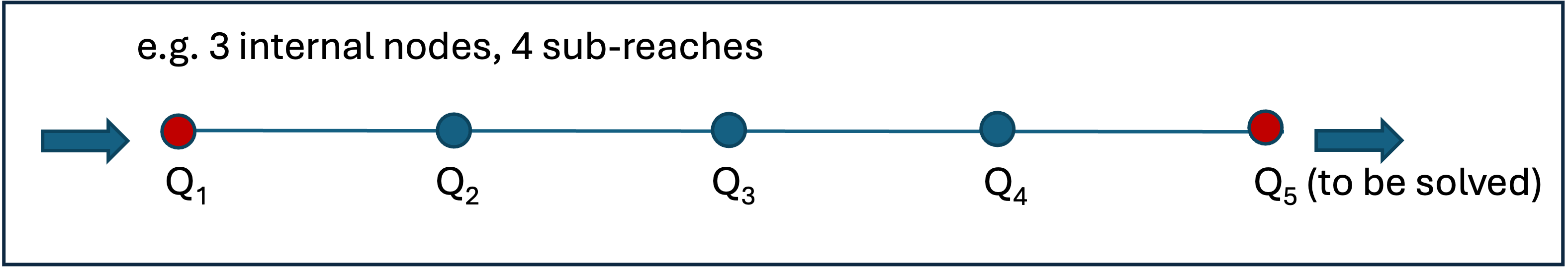
Figure 3.3.5.2 An example of 4 internal nodes per reach.

For example, with 4 internal nodes as shown in, the matrix form of the equations are written as:

(3.3.5.3)\[\small A= \left[ \begin {array}{cccc} 1&0&0&0&0\cr -(\alpha C_{d}+2\beta C_{d})&2+4\beta C_{d}&\alpha C_{a}-2\beta C_{d}&0&0\cr 0&-(\alpha C_{d}+2\beta C_{d})&2+4\beta C_{d}&\alpha C_{a}-2\beta C_{d}&0\cr 0&0&-(\alpha C_{d}+2\beta C_{d})&2+4\beta C_{d}&\alpha C_{a}-2\beta C_{d}\cr 0&0&0&-1&1 \end {array} \right]\]

(3.3.5.4)\[\small Q= \left[ \begin {array}{c} Q_{1}^{t+1} \cr Q_{2}^{t+1} \cr Q_{3}^{t+1} \cr Q_{4}^{t+1} \cr Q_{5}^{t+1} \end {array} \right]\]

(3.3.5.5)\[\small b= \left[ \begin {array}{c} Q_{1}^{t+1} \cr ((1-\alpha)C_{a} + 2(1-\beta)C_{d}) \cdot Q_{1}^{t} + (2-4(1-\beta)C_{d}) \cdot Q_{2}^{t} - ((1-\alpha)C_{a}-2(1-\beta)C_{d}) \cdot Q_{3}^{t} \cr ((1-\alpha)C_{a} + 2(1-\beta)C_{d}) \cdot Q_{2}^{t} + (2-4(1-\beta)C_{d}) \cdot Q_{3}^{t} - ((1-\alpha)C_{a}-2(1-\beta)C_{d}) \cdot Q_{4}^{t} \cr ((1-\alpha)C_{a} + 2(1-\beta)C_{d}) \cdot Q_{3}^{t} + (2-4(1-\beta)C_{d}) \cdot Q_{4}^{t} - ((1-\alpha)C_{a}-2(1-\beta)C_{d}) \cdot Q_{5}^{t} \cr a \cdot dx \end {array} \right]\]

The top row of the system of equations is upstream boundary conditions, which is inflow from upstream reaches (i.e., Dirichlet boundary condition). The Bottom row of the system of equations is downstream boundary condition. Here, Neumann boundary condition, which specifies the gradient of discharge between two adjacent nodes at the downstream end, is used. Neumann boundary condition at the downstream end is written by:

(3.3.5.6)\[\frac{\partial Q}{\partial x}\Big{|}_{x=5}\]

which is discretized as \(Q_{5}^{t+1} - Q_{4}^{t+1} = a \cdot dx\). The gradient at downstream end \(a\) is approximated by the Q computed at the nodes at previous time step.

What makes this numerical solution become kinematic wave solution is simply to set D to zero.